What is NO2?
NO2 is nitrogen dioxide and mostly enters our atmosphere from burning fuel. From cars, trucks, vessels, but also from industrial sites. You can find more information here.
What is O3?
Ground-level ozone, what we breathe, is formed primarily from photochemical reactions between two major classes of air pollutants, volatile organic compounds (VOC) and nitrogen oxides (NOx). You can find more information.
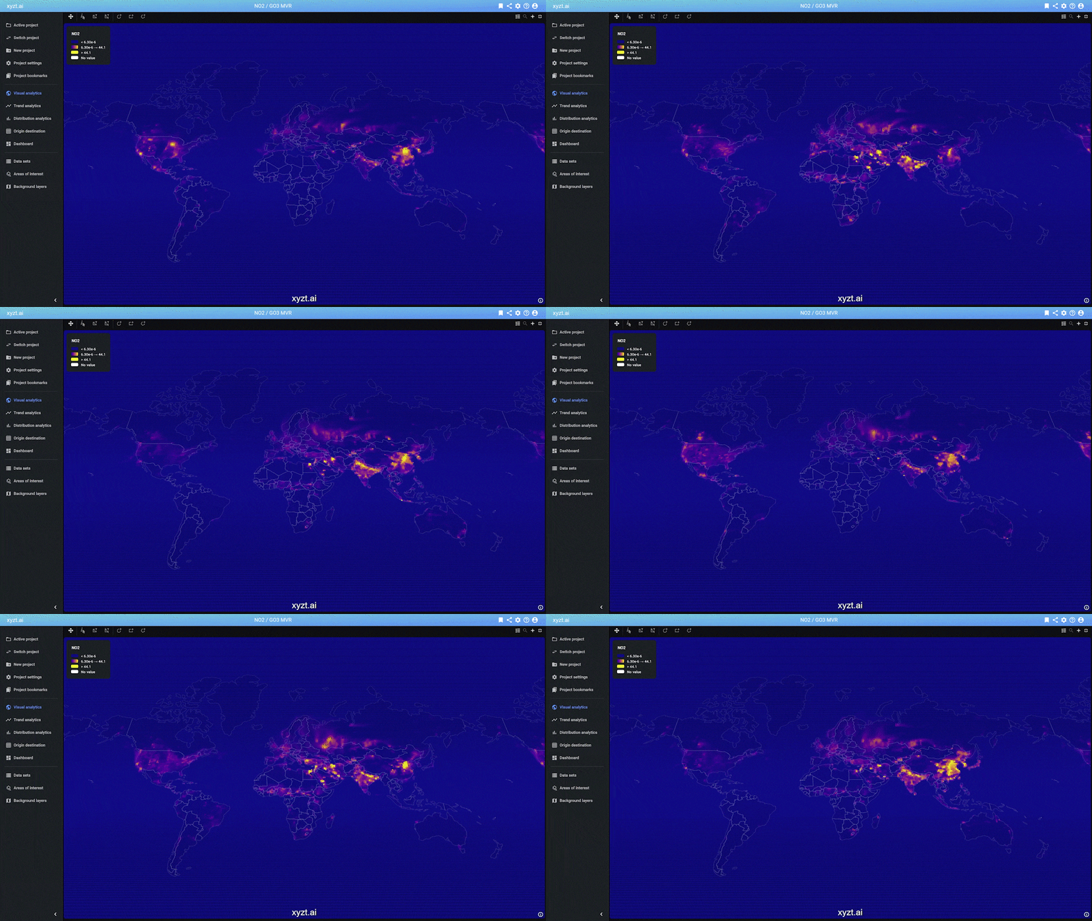
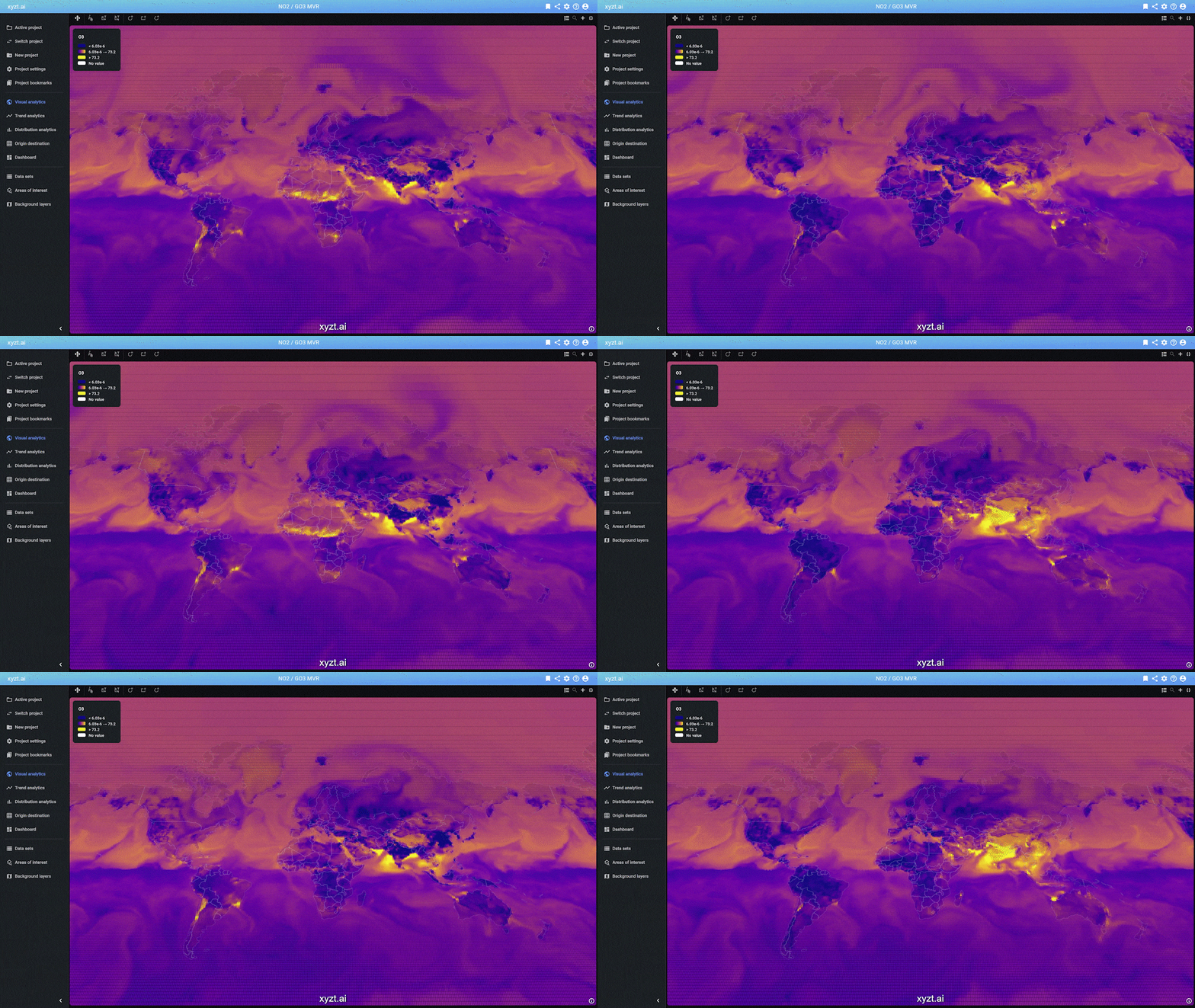
Benefits of using xyzt.ai for analyzing atmospheric data
xyzt.ai is a visual analytics platform that handles any data of the form x,y,z,t,values, meaning that it handles spatio-temporal (multi-variate) data.
So why should you use xyzt.ai for analyzing atmospheric data. The top 5 reasons are:
- It allows you to handle large data sets at different scales in an exploratory manner, allowing you to answer questions quickly and easily.
- It is an interactive tool, allowing you to apply filters, scroll through or animate time, slice the data spatially, temporally, or according to any attribute,… and get immediate feedback, even for gigabytes of data.
- You can answer complex questions such as "Which regions in Europe saw threshold A for NO2 exceeded most during the past month?". It also allows you to combine multiple variables and perform queries on a combination of all, for example answering "Which regions globally, saw the Ozone level exceeding threshold A and the NO2 level exceeding threshold B the most in the past month?"
- It allows you to combine multiple data sets, for example combining atmospheric data with connected car data.
- You can easily share your insights by building dashboards and creating shared links.
Step 1: Obtaining data
The European Copernicus program provides the Atmosphere Monitoring Service where a large number of datasets can be downloaded. You can access the data store here and then search for nitrate dioxide or ozone. Or you can use Google’s data set search using those search terms.
You can select the region, time period, levels and then request a package to download. Most of the data comes in NetCDF format.
What is NetCDF?
Managed by unidata, NetCDF (Network Common Data Form) is a set of software libraries and machine-independent data formats that support the creation, access, and sharing of array-oriented scientific data. It is also a community standard for sharing scientific data. The files have an extension.nc.
Step 2: Preparing the data for the xyzt.ai platform
The xyzt.ai platform does currently not directly support NetCDF files, so we need to convert the data into a well-known format, such as CSV.
How NetCDF data is structured
NetCDF structures data in different variables where each variable has a data type, dimension, and data array. A variable can depend on another variable. For instance, an no2 variable, might depend on a time, a longitude, and a latitude variable.
Here is a printout of a typical Copernicus atmospheric data structure, containing no2 and go3 variables:
float longitude(longitude=480);
 :units = "degrees_east";
 :long_name = "longitude";
float latitude(latitude=241);
 :units = "degrees_north";
 :long_name = "latitude";
int time(time=248);
 :units = "hours since 1900-01-01 00:00:00.0";
 :long_name = "time";
 :calendar = "gregorian";
short no2(time=248, latitude=241, longitude=480);
 :scale_factor = 1.1868220264035013E-11; // double
 :add_offset = 3.8887411517137024E-7; // double
 :_FillValue = -32767S; // short
 :missing_value = -32767S; // short
 :units = "kg kg**-1";
 :long_name = "Nitrogen dioxide mass mixing ratio";
 :standard_name = "mass_fraction_of_nitrogen_dioxide_in_air";
short go3(time=248, latitude=241, longitude=480);
 :scale_factor = 7.116049121989339E-12; // double
 :add_offset = 2.3316447553110163E-7; // double
 :_FillValue = -32767S; // short
 :missing_value = -32767S; // short
 :units = "kg kg**-1";
 :long_name = "Ozone mass mixing ratio (full chemistry scheme)";
 :standard_name = "mass_fraction_of_ozone_in_air";
As can be seen, there are variables for time, longitude, and latitude, and for the two measurement values no2 and go3. time, latitude, and longitude are 1-dimensional, while the others are 3-dimensional arrays, first indexed by time, then latitude, and then longitude.
How xyzt.ai expects data
xyzt.ai expects data in a different format, basically as a linearized list of records, where each record is of the following form:
identifier,time,longitude,latitude,no2,go3
The order of these does not matte
r. The number of measurement variables does not matter either. Every line or record has to have an identifier, a time, a longitude, and a latitude coordinate.
The identifier in this case could be as simple as a constant value or the name of the data set. It should not be unique for every record.
Here is an example extract of a CSV file that can be ingested in the xyzt.ai platform:
0,2020-12-01 01:00:00,90.0,0.0,0.023746440527071533,61.58420495007668
0,2020-12-01 01:00:00,90.0,0.75,0.023746440527071533,61.58420495007668
0,2020-12-01 01:00:00,90.0,1.5,0.023746440527071533,61.58420495007668
0,2020-12-01 01:00:00,90.0,2.25,0.023746440527071533,61.58420495007668
0,2020-12-01 01:00:00,90.0,3.0,0.023746440527071533,61.58420495007668
0,2020-12-01 01:00:00,90.0,3.75,0.023746440527071533,61.58420495007668
0,2020-12-01 01:00:00,90.0,4.5,0.023746440527071533,61.58420495007668
0,2020-12-01 01:00:00,90.0,5.25,0.023746440527071533,61.58420495007668
0,2020-12-01 01:00:00,90.0,6.0,0.023746440527071533,61.58420495007668
0,2020-12-01 01:00:00,90.0,6.75,0.023746440527071533,61.58420495007668
...
Converting the data from NetCDF to CSV
This is a straightforward process going from the more implicitly defined (multi-dimensional) arrays in a NetCDF file, to a linearized more explicit data representation in CSV format.
Since on a daily basis I’m using Java, I will use the netcdf-java software from UCAR to do the conversion. The same can of course be implemented in your preferred language, such as Python.
Step 3: Creating a project and uploading the data
To get the data in the xyzt.ai platform, first create project and add a new data set. Before being able to push your CSV files, you need to define the structure and format of the columns in your data. This can be done through the wizard or by uploading a small data properties file (also in CSV format).
For our converted NetCDF data with no2 and go3 properties, the definition looks like this:
dataset,id:string,identifier,false,0
time,time,time,true,0
latitude,y:double,latitude,true,0
longitude,x:double,longitude,true,0
NO2,double,Nitrogen dioxide volume mixing ratio,true,0.001
O3,double,Ozone volume mixing ratio (full chemistry scheme),true,0.001
The first 4 lines define the mandatory properties, while the last 2 define our custom data properties.
Once the data properties are defined, you must configure the spatial and temporal resolutions (step 3 in the data upload configuration):
- The spatial resolution defines the finest size of the cells in
- which the data is aggregated. This is in meters. For this data set, the resolution of the data is roughly 12.5km, so we take 12500 as the spatial resolution.
- The temporal resolution can be left to the default.
You can now upload the CSV file(s) using drag’n’drop or using the REST API (step 4 in the data configuration process).
Step 4: Visually analyzing the data
You can now visualize and analyze the atmospheric data through the Visual Analytics page. You have access to all dimensions and data properties for styling and filtering:
- Spatially you can zoom in our out of a region or draw a polygon shape to restrict your analysis area.
- Temporally you can fit the timeline on a single measurement instance, or on multiple time instances and do queries and visualizations over longer time periods.
- You can apply filters based on a single property such as for example filtering on data points where NO2 > 40. You can also combine queries on NO2 and O3 using combined filters.
Tip
By default the Visual Analytics page fits on the entire time range and plots a heatmap of the number of records under each pixel. Since in the example above there are 248 time slices, there will also be in most areas 248 records underneath each pixel.Change the time range by dragging one of the vertical lines or zooming in on the timeline and switch to visualize one of the NO3 or NO2 properties. You can also change to a different color map and adjust the value range that is mapped.
Finally, save your setting by creating a bookmark using the bookmark icon in the top right corner.
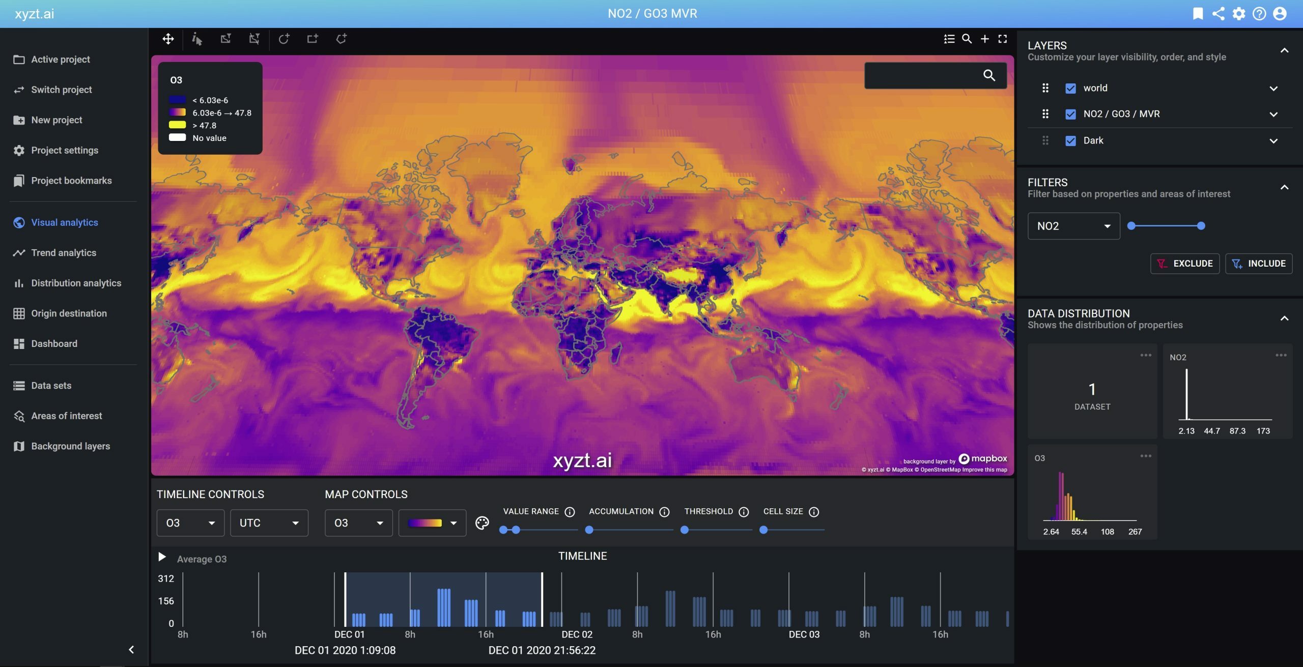
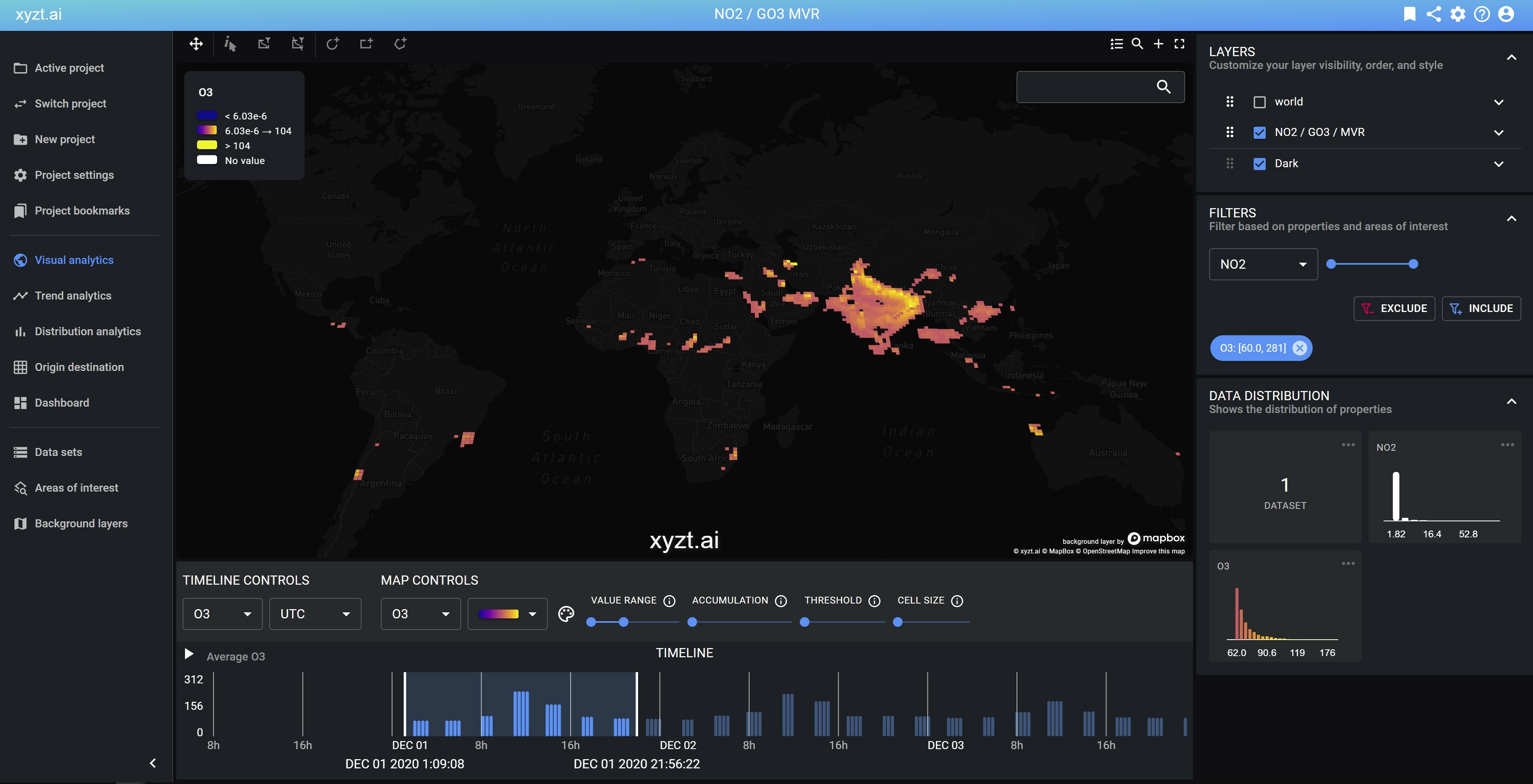
Example 1: Analyzing all regions with O3 levels > 60 ppbv
Follow these steps to look at 1 day of O3 data:
- Switch to visualizing O3 under MAP CONTROLS
- Switch to an appropriate heatmap, for example Plasma
- Zoom in on the timeline and move the vertical lines to fit on one day of data
- Adjust the value range slider to map the required range of O3 levels to the color map. See also the legend.
This results in an image like this:
To filter out all areas where O3 < 60 ppbv, simply apply a filter on the right by
- Selecting O3 in the drop-down box under FILTERS
- Moving the range slider to the required range
- Pressing the INCLUDE button
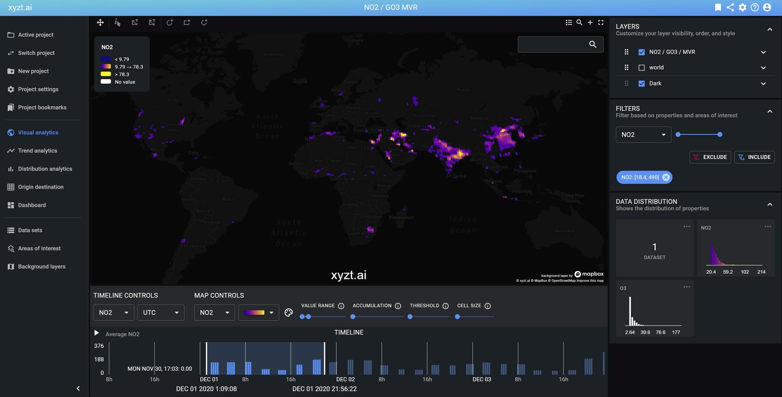
Example 2: All regions with NO2 levels > 18.4 ppbv
Similarly, you can switch to visualizing the NO2 property and applying a filter on the NO2 value.
Example 3: Determining which areas see high NO2 values for many days
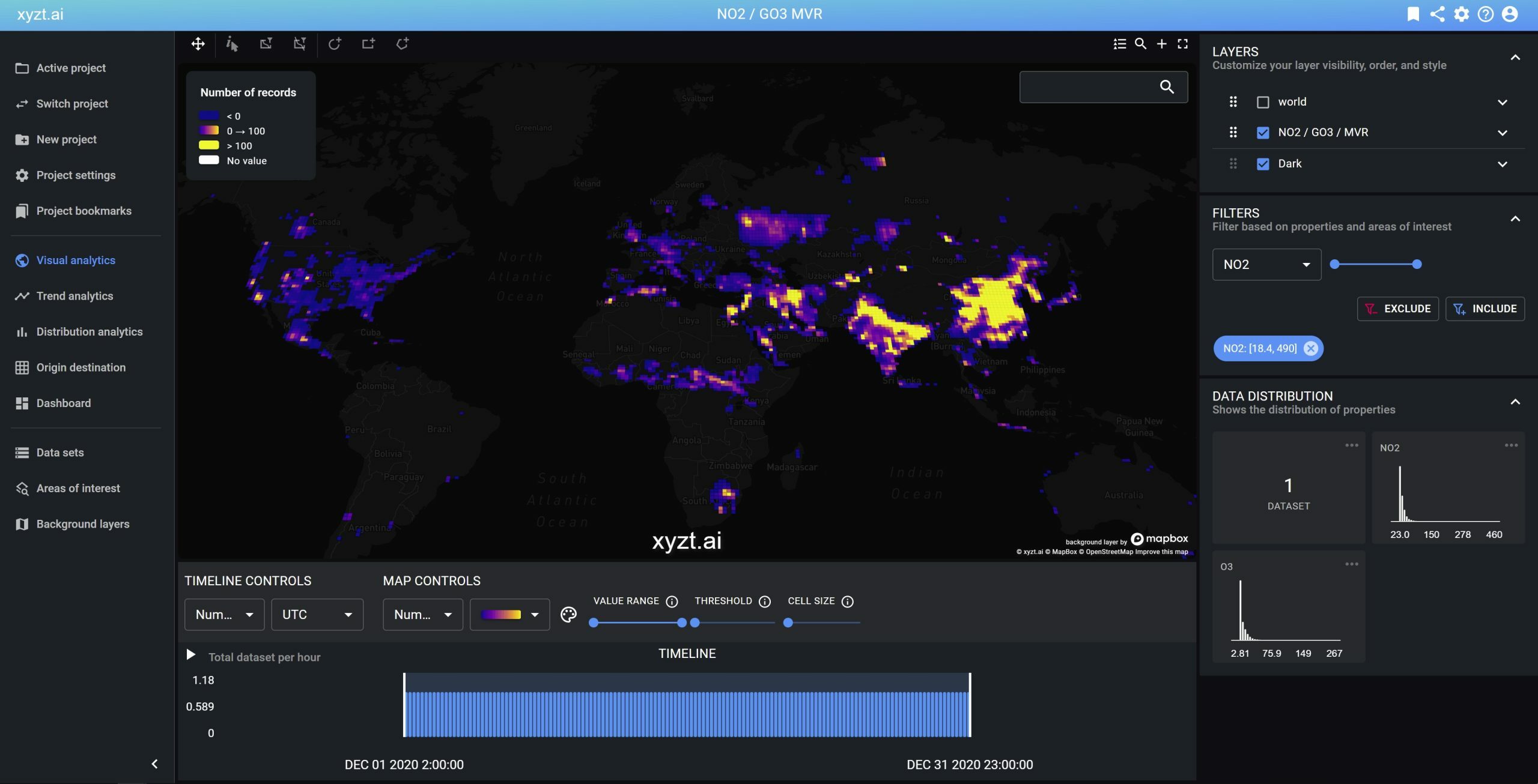
In this analysis we do not want to plot the NO2 values on the map themselves, but instead want to obtain a heatmap of areas where the 18.4 NO2 value threshold is crossed for many days.
This can be obtained as follows:
- Fit the timeline on the entire data set range
- Apply the NO2 > 18.4 filter in the filters panel on the right
- Select "Number of records" under map control
- Select an appropriate heatmap, for example Plasma
The map now shows areas where the NO2 = 18.4 ppbv value is crossed at least once and colors these areas blue. Where the value is crossed many times, the color will be yellow. It looks like India and large parts in China are lighting up very brightly.
Step 5: Sharing your insights
You can share your analysis results with your coworkers or customers in multiple ways:
- The Visual Analytics page can be shared through a shared link, by clicking on the shared link in the top right corner.
- You can bookmark this page and users with an account can access the bookmark.
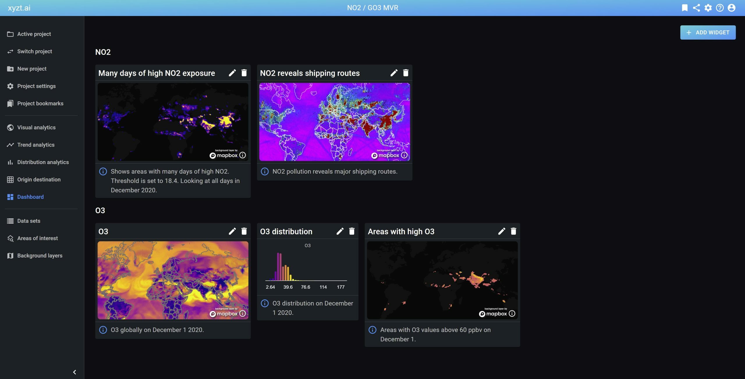
- You can place your maps and widgets on a dashboard and share the dashboard
Conclusion
xyzt.ai is a platform for analyzing anything spatio-temporal. This includes moving things such as vessels, cars, crowds. It also includes measurement (and prediction) values such as atmospheric data, wave data, weather data.
Feel free to reach out for the data sets and conversion code or for a demo.
